Random Variables: Distribution and Expectation¶

约 545 个字预计阅读时间 2 分钟

Random Variables¶

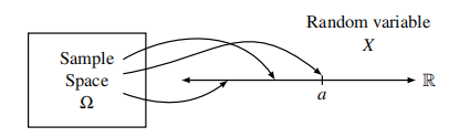
A random variable $X$ on a sample space $\Omega$ is a function $X: \Omega\rightarrow R$ that assigns to each point $\omega\in \Omega$ a real number $X(\omega)$

Note

the term “random variable” is really something of a misnomer: it is a function so there is nothing random about it and it is definitely not a variable!

Probability Distribution¶

When we introduced the basic probability space we defined two things:

The sample space $\Omega$ consisting of all the possible outcomes(sample points) of the experiment.
The probability of each of the sample points

Analogously, there are two important things about any random variable"

The set of values that it can take
The probability with which it takes on the values.

Since a random variable is defined on a probability space, we can calculate these probabilities given the probabilities of the sample points.

Let $a$ be any number in the range of a random variable $X$. Then the set

$\left\{ \omega\in\Omega:X(\omega)=a\right\}$ is an event in the sample space, abbreviated by $X=a$.

Distribution:

The distribution of a discrete random variable $X$ is the collection of values $\left\{ (a,P[X=a]):a\in \mathscr{A}\right\}$, where $\mathscr{A}$ is the set of all possible values taken by $X$.

Note that the collection of events $X=a$ satisfy two important properties:

Any two events $X=a_1,X=a_2$ with $a_1 \ne a_2$ are disjoint.
The union of all these events is equal to the entire sample space $\Omega$

Thus the collection of events form a partition of the sample space.

Bernouli Distribution¶

a random variable which takes value in {0,1}: $$ P[X=i]=\begin{cases}p&i=1\ 1-p&i=0\end{cases} $$

Binomial Distribution¶

\[ P[X=i]=\begin{pmatrix}n\\i\end{pmatrix}p^i(1-p)^{n-i} \]

Hypergeometric Distribution¶

\[ P[Y=k]=\frac{\begin{pmatrix}B\\k \end{pmatrix}\begin{pmatrix}N-B\\n-k\end{pmatrix}}{\begin{pmatrix}N\\n\end{pmatrix}} \]

Note

二项分布有放回，超几何分布无放回

Multiple Random Variables and Independence¶

The joint distribution for two discrete random variable $X,Y$ is the collection of values $\left\{((a,b),P[X=a,Y=b]):a\in \mathscr{A},b\in \mathscr{B}\right\}$, where $\mathscr{A}$ is the set of all possible values taken by $X$ and $\mathscr{B}$ is the set of all possible values taken by $Y$.

When given a joint distribution for $X$ and $Y$, the distribution $P[X=a]$ for $X$ is called the marginal distribution for $X$, and can be found by summing over the values of $Y$, That is:

\[ P[X=a]=\sum_{b\in \mathscr{B}}P[X=a,Y=b] \]

Independence

\[ P[X=a,Y=b]=P[X=a]P[Y=b] \]

Expectation¶

The expectation of a discrete random varaible $X$ is defined as $$ E[X]=\sum_{a\in \mathscr{A}}a\times P[X=a] $$ where the sum is over all possible values taken by the r.v.

Linearity of Expectation¶

For any two random variables $X$ and $Y$ on the same probability space, we have $$ E[X+Y]=E[X]+E[Y] $$ Also, for any constant $c$, we have $$ E[cX]=cE[X] $$

Note

It is only sums and differences and constant multiples of random variables that behave so nicely.

最后更新: 2023年10月23日 09:55:35
创建日期: 2023年10月23日 09:55:35